Chapter 7 Data Wrangling: tidyr
7.1 Overview
Now you have some experience wrangling and working with tidy data. But we all know that not all data that you have are tidy. So how do we make data more tidy? With tidyr.
Objectives
- learn
tidyrwith thegapminderpackage - other wrangling: joins, binding
- practice the RStudio-GitHub workflow
- your turn: use the data wrangling cheat sheet to explore window functions
Resources
These materials borrow heavily from:
7.2 tidyr basics
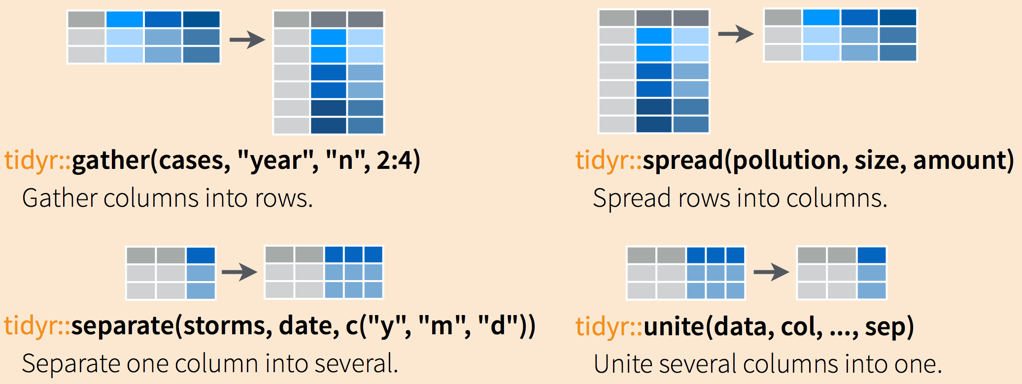
Often, data must be reshaped for it to become tidy data. What does that mean? There are four main verbs we’ll use, which are essentially pairs of opposites:
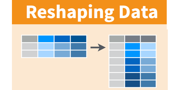
- turn columns into rows (
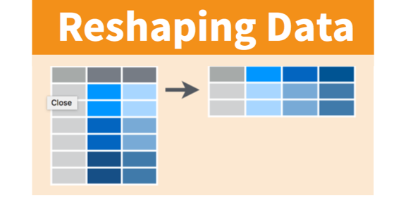
gather()), - turn rows into columns (
spread()), - turn a character column into multiple columns (
separate()), - turn multiple character columns into a single column (
unite())

You use spread() and gather() to transform or reshape data between wide to long formats. long format is the tidy data we are after, where:
- each column is a variable
- each row is an observation
In the long format, you usually have 1 column for the observed variable and the other columns are ID variables.
For the wide format each row is often a site/subject/patient and you have multiple observation variables containing the same type of data. These can be either repeated observations over time, or observation of multiple variables (or a mix of both). Data input may be simpler or some other applications may prefer the ‘wide’ format. However, many of R‘s functions have been designed assuming you have ’long’ format data.
These data formats mainly affect readability. For humans, the wide format is often more intuitive since we can often see more of the data on the screen due to it’s shape. However, the long format is more machine readable and is closer to the formatting of databases. The ID variables in our dataframes are similar to the fields in a database and observed variables are like the database values.
Question: Is gapminder a purely long, purely wide, or some intermediate format?
Sometimes, as with the gapminder dataset, we have multiple types of observed data. It is somewhere in between the purely ‘long’ and ‘wide’ data formats:
- 3 “ID variables” (
continent,country,year) - 3 “Observation variables” (
pop,lifeExp,gdpPercap).
It’s pretty common to have data in this intermediate format in most cases despite not having ALL observations in 1 column, since all 3 observation variables have different units. But we can play with switching it to long format and wide to show what that means (i.e. long would be 4 ID variables and 1 observation variable).
Note: Generally, mathematical operations are better in long format, although some plotting functions actually work better with wide format.
7.2.1 Setup
We’ll work today in RMarkdown. You can either continue from the same RMarkdown as yesterday, or begin a new one.
Here’s what to do:
- Clear your workspace (Session > Restart R)
- New File > R Markdown…, save as something other than
gapminder-wrangle.Rmdand delete irrelevant info, or just continue usinggapminder-wrangle.Rmd
I’m going to write this in my R Markdown file:
Data wrangling with `tidyr`, which is part of the tidyverse. We are going to tidy some data!7.2.2 load tidyverse (which has tidyr inside)
First load tidyr in an R chunk. You already have installed the tidyverse, so you should be able to just load it like this (using the comment so you can run install.packages("tidyverse") easily if need be):
library(tidyverse) # install.packages("tidyverse")7.3 Explore gapminder data — wide format.
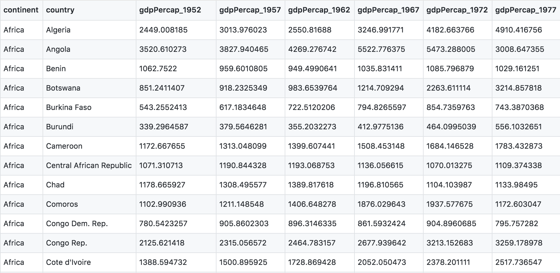
Yesterday we started off with the gapminder data in a format that was already tidy. But what if it weren’t? Let’s look at a different version of those data.
The data are on GitHub. Navigate there by going to:
github.com > ohi-science > data-science-training > data > gapminder_wide.csv
or by copy-pasting this in the browser: https://github.com/OHI-Science/data-science-training/blob/master/data/gapminder_wide.csv
Have a look at the data. You can see there are a lot more columns than the version we looked at before. This format is pretty common, because it can be a lot more intuitive to enter data in this way.

But we want it to be in a tidy way so that we can work with it more easily. So here we go.
7.4 gather() data from wide to long format

Read in the data from GitHub. Remember, you need to click on the ‘Raw’ button first so you can read it directly. Let’s also read in the gapminder data from yesterday so that we can use it to compare later on.
## wide format
gap_wide <- readr::read_csv('https://raw.githubusercontent.com/OHI-Science/data-science-training/master/data/gapminder_wide.csv')

## yesterday's format (intermediate)
gapminder <- readr::read_csv('https://raw.githubusercontent.com/OHI-Science/data-science-training/master/data/gapminder.csv')
Let’s have a look:
head(gap_wide)
str(gap_wide)
While wide format is nice for data entry, it’s not nice for calculations. Some of the columns are a mix of variable (e.g. “gdpPercap”) and data (“1952”). What if you were asked for the mean population after 1990 in Algeria? Possible, but ugly. But we know it doesn’t need to be so ugly. Let’s tidy it back to the format we’ve been using.
Question: let’s talk this through together. If we’re trying to turn the
gap_wideformat intogapminderformat, what structure does it have that we like? And that we want to change?
- We like the continent and country columns. We won’t want to change those.
- For long format, we’d want just 1 column identifying the variable name (
tidyrcalls this a ‘key’), and 1 column for the data (tidyrcalls this the ’value’). - For intermediate format, we’d want 3 columns for
gdpPercap,lifeExp, andpop. - We would like year as a separate column.
Let’s get it to long format. We’ll have to do this in 2 steps. The first step is to take all of those column names (e.g. lifeExp_1970) and make them a variable in a new column, and transfer the values into another column. Let’s learn by doing:
Let’s have a look at gather()’s help:
?gatherQuestion: What is our key-value pair?
We need to name two new variables in the key-value pair, one for the key, one for the value. It can be hard to wrap your mind around this, so let’s give it a try. Let’s name them obstype_year and obs_value.
Here’s the start of what we’ll do:
gap_long <- gap_wide %>%
  gather(key   = obstype_year,
         value = obs_values)
We got a warning message. This means that gather() worked, but maybe not how we wanted it to to.
Although we were already planning to inspect our work, let’s definitely do it now:
str(gap_long)
head(gap_long)
tail(gap_long)
So we have successfully reshaped our dataframe, but really not how we wanted. Very important to check, and listen to that warning message–dropping attributes seems very suspicious.
What went wrong? Notice that it didn’t know that we wanted to keep continent and country untouched; we need to give it more information about which columns we want reshaped. We can do this in several ways.
A good way: identify the columns by name. Listing them out by explicit name can be a good approach if there are a few. But there’s a lot here: over 30. But I’m not going to list them out here, and way too much potential for error if you tried gdpPercap_1952, gdpPercap_1957, gdpPercap_1962… But we could use some of dplyr’s awesome helper functions — because we expect that there is a better way to do this!
gap_long <- gap_wide %>%
  gather(key   = obstype_year,
         value = obs_values,
         dplyr::starts_with('pop'),
         dplyr::starts_with('lifeExp'),
         dplyr::starts_with('gdpPercap'))

str(gap_long)
head(gap_long)
tail(gap_long)
Success! And there is another way that is nice to use if your columns don’t follow such a structured pattern: you can exclude the columns you don’t want.
gap_long <- gap_wide %>%
  gather(key   = obstype_year,
         value = obs_values,
         -continent, -country)

str(gap_long)
head(gap_long)
tail(gap_long)
To recap:
Inside gather() we first name the new column for the new ID variable (obstype_year), the name for the new amalgamated observation variable (obs_value), then the names of the old observation variable. We could have typed out all the observation variables, but as in the select() function (see dplyr lesson), we can use the starts_with() argument to select all variables that starts with the desired character string. Gather also allows the alternative syntax of using the - symbol to identify which variables are not to be gathered (i.e. ID variables).
OK, but we’re not done yet. obstype_year actually contains two pieces of information, the observation type (pop,lifeExp, or gdpPercap) and the year. We can use the separate() function to split the character strings into multiple variables.
?separate –> the main arguments are separate(data, col, into, sep ...). So we need to specify which column we want separated, name the new columns that we want to create, and specify what we want it to separate by. Since the obstype_year variable has observation types and years separated by a _, we’ll use that.
gap_long <- gap_wide %>%
  gather(key   = obstype_year,
         value = obs_values,
         -continent, -country) %>%
  separate(obstype_year,
           into = c('obs_type','year'),
           sep="_")
No warning messages…still we inspect:
str(gap_long)
head(gap_long)
tail(gap_long)
Excellent. This is long format: every row is a unique observation. Yay!
7.4.1 Your turn
Using
gap_long, calculate the mean life expectancy, population, and gdpPercap for each continent. Hint: use thedplyr::group_by()anddplyr::summarize()functionsWhat other helper functions can you use with
dplyr::select()? Would any be useful in our example above? Why or why not?Knit the R Markdown file and sync to Github (pull, stage, commit, push)
# solution (no peeking!)
gap_long %>%
  group_by(continent, obs_type) %>%
    summarize(means = mean(obs_values))
7.5 spread() data from long to intermediate format
Alright! Now just to double-check our work, let’s use the opposite of gather() to spread our observation variables back to the original format with the aptly named spread(). You pass spread() the key and value pair, which is now obs_type and obs_values.

gap_normal <- gap_long %>%
  spread(obs_type, obs_values)
No warning messages is good…but still let’s check:
dim(gap_normal)
dim(gapminder)
names(gap_normal)
names(gapminder)
Now we’ve got an intermediate dataframe gap_normal with the same dimensions as the original gapminder, but the order of the variables is different. Let’s fix that before checking if they are all.equal().
7.5.1 Your turn
Reorder the columns in “gap_normal” to match “gapminder”.
7.5.1.1 Answer (no peeking!)
# one way with dplyr and %>%
gap_normal <- gap_normal %>%
  select(country, continent, year, lifeExp, pop, gdpPercap)

# another way with base R
gap_normal <- gap_normal[,names(gapminder)]
Now let’s check if they are all.equal (?all.equal) is a handy test
all.equal(gap_normal, gapminder)Hmm. Our all.equal() test didn’t pass. Let’s try to figure out why:
head(gap_normal)
head(gapminder)
Ah, they are ordered differently. We’re almost there, the original was ordered by country, continent, then year.
gap_normal <- gap_normal %>%
  arrange(country, continent, year)

all.equal(gap_normal, gapminder)
Better…
str(gap_normal)
str(gapminder)
Mine currently shows that the in gapminder, “year” is an integer (int), but in gap_normal, “year” is a character. So let’s change that and see if that helps:
gap_normal <- gap_normal %>%
  mutate(year = as.integer(year))

all.equal(gap_normal, gapminder)
Hooray!
str(gap_normal)
str(gapminder)
(In the past, mine has shown a slight difference because one is a data.frame and one is a tbl_df, which is similar to a data.frame. We won’t get into this difference now, I’m feeling good about these data sets! We’ve gone from the longest format back to the intermediate and we didn’t introduce any errors in our code.)
7.6 Your turn
Convert “gap_long” all the way back to gap_wide. Hint: you’ll need to create appropriate labels for all our new variables (time*metric combinations) with the opposite of separate:
tidyr::unite().Knit the R Markdown file and sync to Github (pull, stage, commit, push)
7.6.1 Answer (no peeking)
head(gap_long) # remember the columns

gap_wide_new <- gap_long %>%
  # first unite obs_type and year into a new column called var_names. Separate by _
  unite(col = var_names, obs_type, year, sep = "_") %>%
  # then spread var_names out by key-value pair.
  spread(key = var_names, value = obs_values)
str(gap_wide_new)
7.6.2 clean up and save your .Rmd
Spend some time cleaning up and saving gapminder-wrangle.Rmd Restart R. In RStudio, use Session > Restart R. Otherwise, quit R with q() and re-launch it.
This morning’s .Rmd could look something like this:
## load tidyr (in tidyverse)
library(tidyverse) # install.packages("tidyverse")

## load wide data
gap_wide <- read.csv('https://raw.githubusercontent.com/OHI-Science/data-science-training/master/data/gapminder_wide.csv')

head(gap_wide)
str(gap_wide)

## practice tidyr::gather() wide to long
gap_long <- gap_wide %>%
  gather(key   = obstype_year,
         value = obs_values,
         -continent, -country)
# or
gap_long <- gap_wide %>%
  gather(key   = obstype_year,
         value = obs_values,
         dplyr::starts_with('pop'),
         dplyr::starts_with('lifeExp'),
         dplyr::starts_with('gdpPercap'))

## gather() and separate() to create our original gapminder
gap_long <- gap_wide %>%
  gather(key   = obstype_year,
         value = obs_values,
         -continent, -country) %>%
  separate(obstype_year,
           into = c('obs_type','year'),
           sep="_")

## practice: can still do calculations in long format
gap_long %>%
  group_by(continent, obs_type) %>%
  summarize(means = mean(obs_values))

## spread() from normal to wide
gap_normal <- gap_long %>%
  spread(obs_type, obs_values) %>%
  select(country, continent, year, lifeExp, pop, gdpPercap)

## check that all.equal()
all.equal(gap_normal,gapminder)

## unite() and spread(): convert gap_long to gap_wide
head(gap_long) # remember the columns

gap_wide_new <- gap_long %>%
  # first unite obs_type and year into a new column called var_names. Separate by _
  unite(col = var_names, obs_type, year, sep = "_") %>%
  # then spread var_names out by key-value pair.
  spread(key = var_names, value = obs_values)
str(gap_wide_new)
7.6.3 complete: other tidyr awesomeness
For this, let’s look at Jarrett Byrnes’ blog on the topic:
http://www.imachordata.com/you-complete-me/