The following data layers are used in Ocean Health Index global calculations for goal status, trend, pressures, and resilience. Learn how these layers were incorporated into goal calculations on the goals page.

Artisanal fisheries management effectiveness

fp_mora_artisanal

Resilience

Category: ecological/regulatory

Subcategory: fishing

See Artisanal fisheries opportunity data layer for information about data and methods.

Units

scaled 0-1

Artisanal fisheries opportunity

ao_access

This layer represents the opportunity for artisanal and recreational fishing in each country based on the quality of management of the small-scale fishing sector. Global data were extracted from Mora et al. (2009), Figure S4. Figure S4 is based on two expert opinion survey questions related to artisanal and recreational fishing (classified as small-scale fishing; presented in Table S5). Overall scores for small-scale fisheries management for each country are based on a scale of 0 to 100, with higher scores representing better management. These values were then rescaled (using a maximum value of 100 and minimum value of 0) to range between 0 and 1 for each OHI region.

Questions from Mora et al. that were used to evaluate access to artisanal scale fishing:

If recreational fishing exists to any extent, which of the following apply?

Are recreational fishermen required to have a fishing license? Y/N
Are there regulations to the size of fish caught? Y/N
Are there regulations to the number of fish caught? Y/N
Are there regulations to the number of fishermen allowed to fish? Y/N
Are there statistics being collected for this sort of fishing? Y/N

If artisanal fishing exists to any extent, which of the following apply?

Are there regulations to the size of fish caught? Y/N
Are there regulations to the number of fish caught? Y/N
Are there regulations to the number of fishermen allowed to fish? Y/N
Are there statistics being collected for this sort of fishing? Y/N

Units

scaled 0-1

Average species condition

spp_status

See Species goal for calculations.

These are the status data for the species subgoal, calculated using the species model. These data describe the average condition of species within each region based on risk status from the IUCN Red List of Threatened Species (http://www.iucnredlist.org/) and BirdLife International (http://datazone.birdlife.org) data.

We include only species from comprehensively assessed groups (groups with >90% of species assessed) to help control for sampling bias. We found that some regions (e.g., Atlantic) had assessments for a much larger proportion of species than other regions, but this problem was less pronounced when we only included comprehensively assessed species.

These data incorporate regional IUCN assessment information when possible (i.e., when a species’ IUCN status varies geographically).

Units

status score

Average species condition trend

spp_trend

See Species goal for calculations.

These are the trend data for the species subgoal. These data describe changes in species condition within each region based on historical changes in risk status from IUCN Red List of Threatened Species http://www.iucnredlist.org/).

Units

trend score

B/Bmsy estimates

fis_b_bmsy

Status of global fish stocks based on B/Bmsy values (the ratio of population biomass compared to the biomass required to deliver maximum sustainable yield). We preferentially used B/Bmsy estimates from formal stock assessments from the
RAM Legacy Database http://ramlegacy.org/. We assigned the stocks to OHI and FAO regions using Free (2017) spatial data describing the range of each stock. When a stock was missing the most recent years of data, we used linear models of the previous years of data to estimate the missing years.

When RAM data were unavailable, we use the data-limited catch-MSY model (Martell & Frowese 2012) to estimate B/Bmsy values using yearly fish catch reconstruction data. For the catch-MSY model, we defined a stock as a species caught within an FAO major fishing area (www.fao.org/fishery/area/search/en). This definition of a stock eliminated all taxa not identified to species level. This approach assumes that stocks are defined by FAO region, which we know is often not true because multiple stocks of the same species can exist within an FAO region and some stocks cover multiple FAO regions. However, this assumption is necessary without range maps of stocks. The catch data were summed for each species/FAO region/year, and the catch-MSY model was applied to each stock and FAO region to estimate B/Bmsy.

Units

B/Bmsy

Carbon storage weights

element_wts_cs_km2_x_storage

This layer describes the relative value of the habitats in each region to carbon storage, and is calculated by multiplying the habitat extent (km²) in each region by the amount of carbon the habitat sequesters (Laffoley & Grimsditch 2009).

Data is generated in ohi-global/eez/conf/functions.R.

These data are called internally by ohicore functions (see: conf/config.R to see how these data are specified) to weight the data used to calculate pressure and resilience values.

Table 7.3. Carbon storage weights

Habitat	Carbon storage
Mangrove	139
Saltmarsh	210
Seagrass	83

Units

extent*carbon_storage

Chemical pollution

po_chemicals

Pressure

Category: ecological

Subcategory: pollution

This pressure layer is calculated using modeled data for land-based organic pollution (pesticide data), land-based inorganic pollution (using impermeable surfaces as a proxy), and ocean pollution (shipping and ports). These global data are provided at ~1km resolution, with raster values scaled from 0-1 (Halpern et al. 2008, 2015). To obtain the final pressure values, the three raster layers were summed (with cell values capped at 1).

Land-based organic pollution

Data were calculated using modeled plumes of land-based pesticide pollution that provide intensity of pollution at 1km² resolution (Halpern et al. 2008).

Organic pollution was estimated from FAO data on annual country-level pesticide use (http://faostat3.fao.org/faostat-gateway/go/to/browse/R/*/E), measured in metric tons of active ingredients. FAO uses survey methods to measure quantities of pesticides applied to crops and seeds in the agriculture sector, including insecticides, mineral oils, herbicides, fungicides, seed treatments insecticides, seed treatments fungicides, plant growth regulators and rodenticides. Missing values were estimated by regression between fertilizer and pesticides when possible, and when not possible with agricultural GDP as a proxy. Data were summed across all pesticide compounds and reported in metric tons. Upon inspection the data included multiple 0 values that are most likely data gaps in the time-series, so they were treated as such and replaced with NA. In addition, regions with only 1 data point and regions where the most recent data point was prior to 2005 were excluded. Uninhabited countries were assumed to have no pesticide use and thus excluded.

Region-level pollution values were then dasymetrically distributed over a region’s landscape using global landcover data from 2009, derived from the MODIS satellite data at ~500m resolution. These values were then aggregated by ~140,000 global basins, and diffusive plumes were modeled from each basin’s pourpoint. The final non-zero plumes (about ~76,000) were aggregated into ~1km Mollweide (wgs84) projection rasters to produce a single plume-aggregated pollution raster.

These raw values were then ln(X+1) transformed and normalized to 0-1 by dividing by the 99.99th quantile of raster values across all years. The zonal mean was then calculated for each region.

Land-based inorganic pollution

These data are from Halpern et al. (2008, 2015), and available from Knowledge Network for Biocomplexity (KNB, https://knb.ecoinformatics.org/#view/doi:10.5063/F19021PC, rescaled_2013_inorganic_mol). Non-point source inorganic pollution was modeled with global 1 km² impervious surface area data http://www.ngdc.noaa.gov/dmsp/ under the assumption that most of this pollution comes from urban runoff. These data will not capture point-sources of pollution or nonpoint sources where paved roads do not exist (e.g., select places in developing countries). Values were aggregated to the watershed and distributed to the pour point (i.e., stream and river mouths) for the watershed with raster statistics (i.e., aggregation by watershed).

Ocean pollution (shipping lanes, ports)

These data are from Halpern et al. (2015), and available from the Knowledge Network for Biocomplexity (KNB, https://knb.ecoinformatics.org/#view/doi:10.5063/F1DR2SDD, rescaled_2013_one_ocean_pollution_mol). Ocean-based pollution combines commercial shipping traffic data and port data.

Shipping data was obtained from two sources: (1) Over the past 20 years, 10-20% of the vessel fleet has voluntarily participated in collecting meteorological data for the open ocean, which includes location at the time of measurement, as part of the Volunteer Observing System (VOS). (2) In order to improve maritime safety, in 2002 the International Maritime Organization SOLAS agreement required all vessels over 300 gross tonnage (GT) and vessels carrying passengers to equip Automatic Identification System (AIS) transceivers, which use the Global Positioning System (GPS) to precisely locate vessels.

Port data was based on the volume (measured in tonnes) of goods transported through commercial ports as a proxy measure of port traffic. Total cargo volume data by port was collected from regional and national statistical organizations, and from published port rankings.

Units

scaled 0-1

Chemical pollution trend

cw_chemical_trend

See description for Chemical pollution layer.

The inverse of the pressure data (1 - Coastal chemical pollution) was used to estimate chemical trends for the clean water goal. The proportional yearly change in chemical pressure values were estimated using a linear regression model of the most recent five years of data (i.e., slope divided by value from the earliest year included in the regression model). The slope was then multiplied by five to get the predicted change in 5 years.

The only layer with yearly data was land-based organic pollution (pesticide data). The land-based inorganic pollution (using impermeable surfaces as a proxy) and ocean pollution (shipping and ports) remained the same across years.

Units

trend

CITES signatories

g_cites

Resilience

Category: ecological/regulatory

Subcategory: goal

Contracting parties to the Convention on International Trade in Endangered Species of Wild Fauna and Flora (CITES, http://www.cites.org/eng/ disc/parties/alphabet.php). The Convention is an international agreement between governments that aims to ensure that any international trade in plants and animals “does not threaten their survival.” All countries party to the Convention are given full credit for membership (territories are given the same score as their administrative countries); those countries that are not contracting parties are given no credit (score = 0).

Units

0 or 1

Coastal chemical pollution

po_chemicals_3nm

Pressure

Category: ecological

Subcategory: pollution

See description for Chemical pollution.

Methods follow those described for the Chemical pollution layer. However, the rescaled data were clipped to include only pixels within 3nm offshore, and the zonal mean for each region was calculated using this subset of data.

For the clean waters goal calculations, the inverse of the pressure values is used (1 minus chemical pressure).

Units

scaled 0-1

Coastal nutrient pollution

po_nutrients_3nm

Pressure

Category: ecological

Subcategory: pollution

See description for Nutrient pollution.

Methods follow those described for the Nutrient pollution layer. However, the rescaled data were clipped to include only pixels within 3nm offshore, and the zonal mean for each region was calculated using this subset of data.

For the clean waters goal calculations, the inverse of the pressure values is used (1 minus nutrient pressure).

Units

scaled 0-1

Coastal protected marine areas (fishing preservation)

fp_mpa_coast

Resilience

Category: ecological/regulatory

Subcategory: fishing

These data are calculated using the lasting special places status subgoal model using total marine protected area (km²) within 3 nm offshore (see Offshore coastal protected areas layer for information about the data). Following the lasting special places model, a reference point of 30% is used, such that any region with 30%, or more, protected area receives a score of 1.

Units

scaled 0-1

Coastal protected marine areas (habitat preservation)

hd_mpa_coast

Resilience

Category: ecological/regulatory

Subcategory: habitat

See Coastal protected marine areas (fishing preservation) for information about this layer.

Units

scaled 0-1

Coastal protection weights

element_wts_cp_km2_x_protection

This layer describes the relative value of the habitats in each region to coastal protection, and is calculated by multiplying the habitat extent (km²) in each region by the habitat protection rank.

Data is generated in ohi-global/eez/conf/functions.R.

These data are called internally by ohicore functions (see: conf/config.R to see how these data are specified) to weight the data used to calculate pressure and resilience values.

Table 7.4. Coastal protection ranks

Habitat	Protection rank
Coral	4
Mangrove	4
Seaice (shoreline)	4
Saltmarsh	3
Seagrass	1

Units

extent*rank_protection

Coral harvest pressure

hd_coral

Pressure

Category: ecological

Subcategory: habitat destruction

The total tonnes of coral harvest were determined for each region using export data from the FAO Global Commodities database. The tonnes of ornamental fishing was divided by the area of coral, taken from the hab_coral layer, to get the intensity of coral harvest per region. Following this, we set the reference value as the 95th quantile of coral harvest intensity. We then divided the intensity by the reference intensity. Anything that scored above 1 received a intensity pressure score of 1. To incorporate the health of the coral, we then multiplied the intensity pressure score by the health of the coral, to get the final pressure score.

Units

scaled 0-1

Economic diversity

li_sector_evenness

Resilience

Category: social

Sector evenness was measured using Shannon’s Diversity Index, a common measure of ecological and economic diversity that has been applied previously to economic sectors [@attaran_industrial_1986]. The Diversity Index is computed as \({ H }^{ ' }/{ H }_{ max }\) where:

\[ { H }^{ ' } = \sum _{ i }^{ z }{ { f }_{ i }\ast } \ln { { (f }_{ i }) }, (Eq. 7.1) \]

and Z is the total number of sectors, \(fi\) is the frequency of the ith sector (the probability that any given job belongs to the sector), and \(H_{max} = \ln { Z }\).

Units

scaled 0-1

Economic need for artisanal fishing

ao_need

These data are used to estimate the need for artisanal fishing opportunities given teh purchasing power parity adjusted per capita gross domestic product (ppppcgdp) in “constant” USD (World Bank, http://data.worldbank.org/indicator/NY.GDP.PCAP.PP.KD). The World Bank defines gdp as the gross value of all resident producers in the economy plus product taxes and minus and subsidies not included in the value of the products. The gdp is adjusted by population size to get per capita output and by purchasing power parity (ppp) to account for the difference in exchange rates between countries. ppppcgdp data were rescaled to values between zero and one by taking the natural log of the values and dividing by the 99th quantile value across all years/regions (2005 to most recent year).

When a region is missing some years of data, a within region linear model is used to estimate the missing values.

This is actually a measure of prosperity, but it is converted to need in the artisanal opportunities goal model (1 minus ppppcgdp).

Units

scaled 0-1

Economic status scores

eco_status

This layer provides calculated status values for the economies subgoal. Economies is calculated using revenue data from marine sectors.

Note: These data are no longer supported. Consequently, this layer was last updated in 2013, and this goal will no longer be updated with these data.

Economies status is calculated as: (cur_base_value / ref_base_value) / (cur_adj_value / ref_adj_value)

Where, cur_base_value is the most recent revenue values for each sector/region, and ref_base_value is the earliest year of revenue data for each sector/region. These values are adjusted by dividing by the GDP of corresponding region/year to control for larger economic trends. National GDP data were obtained from the World Bank (http://data.worldbank.org/indicator/ NY.GDP.MKTP.CD). For the three EEZs that fall within the China region (China, Macau, and Hong Kong), we combined the values using a population-weighted average.

This layer includes yearly data for revenue in commercial fishing, aquarium trade fishing, mariculture, marine mammal watching, marine renewable energy, and, tourism. The data sources and methods for each sector are described below.

Aquarium trade fishing

To approximate revenue from aquarium fishing we used export data from the FAO Global Commodities database for ‘Ornamental fish’ for all available years. We used data from two of the four subcategories listed, excluding the subcategory ‘Fish for culture including ova, fingerlings, etc.’ because it is not specific to ornamental fish, and the subcategory ‘Ornamental freshwater fish’ because it is not from marine systems.

Commercial fishing

Revenue data for commercial fishing were obtained from FAO’s FishStat database, which provides yearly dollar values of commercial fisheries production for marine, brackish and freshwater species starting in 1950 and updated yearly. To isolate production values attributable to marine and brackish aquaculture, data pertaining to freshwater species were omitted. This species classification process was very time consuming as each species had to be queried individually per year. There was little year-to year variation, and thus data were extracted in 5 year increments, providing data for 1997, 2002 and 2007.

Mariculture

Data on revenues from marine aquaculture were derived from FAO’s FishStat database, which includes country-level data on total production values for marine, brackish, and freshwater species beginning in 1984 and updated yearly. To isolate production values attributable to marine and brackish aquaculture, data pertaining to freshwater species were omitted. This species classification process was very time consuming as each species had to be queried individually per year. There was little year-to year variation, and thus data were extracted in 5 year increments, providing data for 1997, 2002 and 2007.

Marine mammal watching

IFAW provides country-level data on total expenditures (including direct and indirect) attributable to the whale watching industry (O’Connor et al. 2009). Here, total expenditures are used as a close proxy for total revenue. We used total expenditure data (direct and indirect expenditures) to avoid using a literature derived multiplier effect. When IFAW reported “minimal” revenue from whale watching, we converted this description to a 0 for lack of additional information. For countries with both marine and freshwater cetacean viewing, we adjusted by the proportion of marine revenue as described for the jobs dataset.

Marine renewable energy

The United Nations Energy Statistics Database provides production data, in kilowatt-hours (KWh), for tidal and wave electricity. However, only two countries, France and Canada, have high enough levels of production to be reported in this data source. For Canada, production data were replaced with production data (Gross Megawatt hours per year from 1995-2010) provided directly from the Annapolis tidal power plant because the plant provided a longer time series (Ruth Thorbourne, personal communication, Aug 9, 2011). To convert production data into revenue, production values were multiplied by average yearly prices of electricity per KWh specific to Canada and France, provided by the US Energy Information Administration (http://www.eia.gov/emeu/international/elecprii.html; updated June 2010) after conversion to 2010 USD. Some of the production data could not be used because there were no available electricity price data to convert production into revenue, truncating our time series.

Tourism

WTTC reports dollar values of visitor exports (spending by foreign visitors) and domestic travel and tourism spending; combining these two data sets creates a proxy for total travel and tourism revenues. WTTC was chosen as the source for tourism revenue data because of the near-complete country coverage, the yearly time series component starting in 1988 and updated yearly, and the inclusion of both foreign and domestic expenditures. This dataset lumps inland and coastal/marine revenues, and so was adjusted by the percent of a country’s population within a 25 mile inland coastal zone. We included no projected data. We used total contribution to GDP data (rather than direct contribution to GDP) to avoid the use of literature derived multiplier effects.

Units

status 0-100

Economic trend scores

eco_trend

See Economic status scores layer for more information about data and methods.

This layer provides calculated trend values for the economies subgoal. Economies is calculated using revenue data from marine sectors.

Note: These data are no longer supported. Consequently, this layer was last updated in 2013, and this goal will no longer be updated with these data.

Units

trend -1 to 1

EEZ protected marine areas (fishing preservation)

fp_mpa_eez

Resilience

Category: ecological/regulatory

Subcategory: fishing

These data are calculated using the lasting special places status subgoal model (except this calculation is based on the entire eez region vs. 3 nm offshore), using the total marine protected area (km²) within the offshore eez region (see the Offshore coastal protected areas layer for information about the data). Following to the lasting special places model, a reference point of 30% is used, such that any region with 30%, or more, protected area receives a score of 1.

Units

scaled 0-1

EEZ protected marine areas (habitat preservation)

hd_mpa_eez

Resilience

Category: ecological/regulatory

Subcategory: habitat

See EEZ protected marine areas (fishing preservation) for information about this layer.

Units

scaled 0-1

Exposure of ornamental fishing to coral and rocky reef habitats

np_exposure_orn

Exposure is the ln-transformed intensity of harvest calculated as tonnes of harvest per km² of coral and rocky reef of ornamental fishing, relative to the global maximum. We ln transformed the harvest intensity scores because the distribution of values was highly skewed; because we do not know the true threshold of sustainable harvest, nearly all values would be considered highly sustainable without the log transformation. To estimate rocky reef extent area (km²) we used data from Halpern et al. (2008), which assumes rocky reef habitat exists in all cells within 1 km of shore. Coral extent area (km²) are from UNEP-WCMC et al. (2018).

Units

scaled 0-1

Fish oil and fish meal score

np_fofm_scores

Fish oil and fish meal scores from Global Fisheries Landing Data (Watson 2019) and the RAM Legacy Database http://ramlegacy.org/. For this layer, nearly identical methods were used as in the fisheries sub-goal calculations. Instead of producing scores for all global fish stocks, we only produced scores for those that contribute to fish oil and fish meal (Froehlich 2018). The tonnes of harvest of these species were multiplied by 0.7 to reflect the proportion of this catch used for oil or feed.

Units

scaled 0-1

Fisheries management index

fp_fish_management

These data describe the current effectiveness of fisheries management regimes along 6 axes (Melnychuk et al. 2017): scientific robustness, policy transparency, implementation capacity, subsidies, fishing effort, and foreign fishing. All countries with coastal areas were assessed through a combination of surveys, empirical data and enquiries to fisheries experts. For each OHI reporting region, scores for each category were rescaled between 0 and 1 using the maximum possible value for each category and then the average score of all 6 categories was used as the overall fisheries management effectiveness score.

Data are not accessible in csv format from website, so points were manually entered into excel and saved as a csv. Because FMI scores only exist for 40 out of the 220 OHI regions, we predicted missing values using a linear models with Social Progress Index and UN georegion data as predictors. Uninhabited regions (N=20) were given an NA value.

Units

scaled 0-1

Fishery catch data

fis_meancatch

Fisheries catch data describe the average catch across years (from 1980 to present) for each fish stock and region. We have traditionally included all fisheries catch in the Food Provision goal. However, a substantial portion of the catch is not used for human consumption, but rather for fish oil and fish meal used primarily for animal feed. To account for this, we excluded the proportion of catch that produce fish oil and fish meal for animal feed (0.9) from the total catch. These values were used to weight stock status scores (derived from B/Bmsy values) in the fisheries model. The Global Fisheries Landings data (Watson 2019) is reported at 0.5 degree resolution for taxonomic levels range from species to class to “Miscellaneous not identified” for each year. Tonnes of catch for each taxon and year were summed within each OHI region, and then the average catch across years (1980 to present) was determined for each taxon and region.

Units

tonnes

Food provision weights

fp_wildcaught_weight

To weight the relative contributions of fisheries and mariculture to the food provision goal, we calculate the tonnes of fisheries production relative to the total tonnes of food production from fisheries and mariculture.

Units

proportion

Genetic escapes

sp_genetic

Pressure

Category: ecological

Subcategory: nonindigenous species

This layer represents the potential for harmful genetic escapement based on whether the species being cultured is native or introduced. Data come from the Monterey Bay Aquarium Seafood Watch Aquaculture Recommendations (SFW, 2020). Ten mariculture practice criteria from the Monterey Bay Aquarium Seafood Watch (SFW) Aquaculture Recommendations contributed to the sustainability of mariculture (data quality, effluent, habitat risk, chemical use, feed, escapes, disease, source of stock, predator and wildlife mortalities, and escape of secondary species). The escapes criteria was used for this layer, where a score of 1 is the lowest, and a score of 10 is the highest. The scores reflect the potential impact of genetic escapes on local biodiversity, if these species were to escape. Genetic ‘pollution’ can arise when larvae, spats or seeds escape from poorly managed hatcheries, making native species vulnerable to outbreeding depressions and/or genetic bottlenecks. All country average scores were then rescaled from 0 to 1 using the maximum possible raw SFW score of 10 and minimum of 1.

These scores are country and species-specific, however, many country/species combinations are not assessed by SeaFood Watch. Given that each mariculture record must have a corresponding escapes score we used a series of steps to estimate escapes scores for every country and species. If a country/species match was available we used that, otherwise, we gapfilled using the following sequence:

Used the global species value provided by SeaFood Watch
Within a country, used average of species within the same family
Within a UN geo-political region, used average of species within the same family
Global, use average of species within the same family
Global, use average of species within a broad taxonomic grouping (e.g., crustaceans, algae, bivalves, etc.)
Finally, if these scores were not available for the categories above, we used the global average of all species.

Seaweed or algae species were given the global seaweed escapes score provided by the Seafood Watch recommendations. We are aware that there is some bias associated with using scores derived as averages across countries because they were originally assigned to specific species-country pairs, nevertheless this is preferable to applying an escapes score solely based on a subset of the species harvested.

Units

scaled 0-1

Global Competitiveness Index (GCI)

li_gci

Resilience

Category: social

The World Economic Forum’s Global Competitiveness Index (GCI) provides a country level assessment of competitiveness in achieving sustained economic prosperity (Schwab 2011, http://gcr.weforum.org). The GCI is a weighted index based on 12 pillars of economic competitiveness: institutions, infrastructure, macroeconomic environment, health and primary education, higher education and training, goods market efficiency, labor market efficiency, financial market development, technological readiness, market size, business sophistication, and innovation. The GCI can in theory span from 1 to 7, based on this range, we rescaled the scores to range between 0 and 1. Uninhabited OHI regions are given an NA score.

Units

scaled 0-1

Habitat condition of coral

hab_coral_health

See Habitat extent of coral layer for more information.

Coral condition was calculated using current condition data divided by reference condition. We used condition data from percent live coral cover from 12,634 surveys from 1975-2006 (Bruno and Selig 2007, Schutte et al. 2010). When multiple data points were available for the same site and year, we averaged these data, and also averaged the site data to calculate a per country per year average. However, data were missing for several countries and some countries did not have data for the reference or current year time periods or had only 1-2 surveys. Because coral cover can be highly temporally and spatially dynamic, having only a few surveys that may have been motivated by different reasons (i.e., documenting a pristine or an impacted habitat) can bias results. To calculate condition we used fitted values from a linear trend of all data per country, which was more robust to data poor situations and allowed us to take advantage of periods of intense sampling that did not always include both current and reference years. Then, we created a fitted linear model of all these data points from 1975-2010, provided that 2 or more points are in 1980-1995 and 2 or more points are in 2000-2010. We defined the ‘current’ condition (health) as the mean of the predicted values for 2008-2010, and the reference condition as the mean of the predicted values for 1985-1987. Where country data were not available, we used an average from adjacent EEZs weighted by habitat area, or a georegional average weighted by habitat area, based on countries within the same ocean basin (Figure 7.1).

Figure 7.1. Georegions to gapfill coral reef data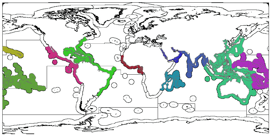

Units

proportion

Habitat condition of mangrove

hab_mangrove_health

See Habitat extent of mangrove layer for more information.

Mangrove condition was defined as the current cover divided by reference cover. FAO mangrove area data was provided on a country basis for 1980, 1990, 2000, and 2005. Current condition is based on 2005 cover, and reference condition is based on the 1980 cover.

Units

proportion

Habitat condition of saltmarsh

hab_saltmarsh_health

See Habitat extent of saltmarsh layer for more information.

Salt marsh condition was based on trends in salt marsh area for regions where both a current and reference data year were available. An increasing or stable trend was assigned condition = 1.0, and a decreasing trend was assigned condition = 0.5. Data was from multiple sources (Bridgham et al. 2006, Dahl 2011, Ministry for the Environment 2007, JNCC 2004, EEA 2008).

Units

proportion

Habitat condition of seagrass

hab_seagrass_health

See Habitat extent of seagrass layer for more information.

Seagrass condition was calculated on a per-site basis from Waycott et al. (2009), which provides seagrass habitat extent data for several sites around the world over several years. Reference condition was calculated as the mean of the three oldest years between 1975-1985, or the two earliest years if needed. If data meeting these conditions was not available, we fitted a linear model to all data points, and then used the mean of the predicted values for 1979-1981 as the reference condition. For the current condition we used the mean of the three most recent years after 2000 or the two most recent years. If condition data satisfying these constraints were still not available, we fitted a linear model to all data points, provided that there were at least three data points and then used the mean of the predicted values for 2008-2010 as the current condition and the mean of the predicted values for 1979-1981 as the reference condition. Otherwise, we used neighboring (adjacent) regional averages, weighted by habitat area, or averages weighted by habitat area using seagrass geographical regions as defined by Hemminga and Duarte (2000). We did not project beyond a 15-year timeframe.

Units

proportion

Habitat condition of seaice

hab_seaice_health

See Habitat extent of seaice layer for more information.

Sea-ice condition was calculated using sea-ice concentrations from the USA National Snow and Ice Data Center (Cavalieri et al. 2014; https://nsidc.org/cryosphere/quickfacts/seaice.html) as the current percent cover of sea-ice (average of 3 years of data) divided by the average historical percent cover, defined as the start of the data (1979) until the year 2000 as recommended by the National Snow & Ice Data Center for both sea-ice edge and sea-ice shoreline habitats.

Units

proportion

Habitat condition of softbottom

hab_softbottom_health

See Habitat extent of softbottom layer for more information.

Soft bottom subtidal habitat condition was estimated using relative intensity of fishing with demersal destructive gear types. We used global catch data (Watson 2019) that describes the tonnes of harvest for each species and gear type at 0.5 degree raster scale. To estimate the amount of destructive catch, we multiplied each catch record by a value, ranging from 0-1 (1 being the most destructive), based on how destructive the gear type is to soft bottom habitat (trawl and dredge = 1, gillnet and trap = 0.5, “other” = 0.25, and midwater trawl, pole and line, longline, purse seine and seine = 0).

We summed commercial and non-commercial destructive catch for each OHI region and year, and we divided by the area of soft-bottom habitat in the region. The extent of soft-bottom area within a region was defined as shallow subtidal (0-60m) and outer shelf (60-200m) soft bottom habitat. Because these values were extremely skewed, we \(ln(X+1)\) transformed them and then rescaled by dividing by the 99th quantile of density across all years/regions. Condition was then calculated as one minus the rescaled catch density in the most recent year and further rescaled to the median condition value across all years. Any value greater than the median was set = 1.0.

Units

proportion

Habitat condition trend of coral

hab_coral_trend

See Habitat extent of coral layer for more information.

Coral trend was calculated using condition data from 1975-2006 (Bruno and Selig 2007, Schutte et al. 2010).

Units

trend

Habitat condition trend of mangrove

hab_mangrove_trend

See Habitat extent of mangrove layer for more information.

We used Hamilton and Casey’s (2016) mangrove cover data to estimate the proportional yearly change in mangrove area using a linear regression model of the most recent five years of data (i.e., slope divided by data from the earliest year included in the regression model). The slope was then multiplied by five to get the predicted change in 5 years. The original mangrove data are provided yearly (2000-2012) at 30m raster cell resolution (with the estimated area of mangrove cover in each cell).

Units

trend

Habitat condition trend of saltmarsh

hab_saltmarsh_trend

See Habitat extent of saltmarsh layer for more information.

General trends in salt marsh area were determined from 1994-2007 using data from multiple sources (Bridgham et al. 2006, Dahl 2011, Ministry for the Environment 2007, JNCC 2004, EEA 2008). For trend estimates, we extracted categorical condition data (‘increasing”, “stable”, “declining” score as 0.5, 0.0, and -0.5, respectively) from these sources on a per country basis when both a current and reference data year were available.

Units

trend

Habitat condition trend of seagrass

hab_seagrass_trend

See Habitat extent of seagrass layer for more information.

Trend in seagrass condition was determined using two data sources (Waycott et al. 2009, Short et al. 2010). Short et al. (2010) measured percent cover on a per sample, per site, per year basis, whereas Waycott et al. (2009) measured habitat area on a per site, per year basis. We used data from Short if there were at least 3 data points between 2001-2010. If this condition was not met, we calculated trends from Waycott for the most recent 10 years after 1990 or else we used the mean of the trend in the adjacent regions or the regions within the corresponding seagrass geographical regions using the same methods described above for the in status.

Units

trend

Habitat condition trend of seaice

hab_seaice_trend

See Habitat extent of seaice layer for more information.

Trends for sea-ice edge and sea-ice shoreline habitats were calculated using sea-ice concentrations from the USA National Snow and Ice Data Center (Cavalieri et al. 2014; https://nsidc.org/cryosphere/quickfacts/seaice.html). The average yearly proportional change in extent was estimated using a linear regression model that included the most recent five years of data (e.g., slope estimate was divided by the extent for earliest year included in the regression model), and this value was multiplied by five to get the predicted change in 5 years. Each year of data represents a 3-year average, to smooth yearly variation.

Units

trend

Habitat condition trend of softbottom

hab_softbottom_trend

See Habitat extent of softbottom layer for more information.

Trend in soft bottom subtidal condition was estimated using a linear regression model that included the most recent five years of condition data. The proportional change in condition was determined (e.g., slope estimate was divided by the condition value for earliest year included in the regression) and then multiplied by five to get the change predicted in 5 years.

Units

trend

Habitat extent of coral

hab_coral_extent

Coral data are used to calculate coastal protection goal, habitat subgoal, and exposure variable of the natural products goal.

Coral extent area (km²) are derived from the dataset Global Distribution of Coral Reefs .

Units

km2

Habitat extent of mangrove

hab_mangrove_extent

Mangrove data are used to calculate the coastal protection and carbon storage goals, and the habitat subgoal.

Hamilton and Casey’s (2016) yearly (2000-2012) mangrove cover data were used to calculate mangrove extent (km²). Data were provided at 30m raster cell resolution (with the estimated area of mangrove cover in each cell) which we converted to 500m resolution to facilitate global calculations.

Units

km2

Habitat extent of rocky reef

hab_rockyreef_extent

Rocky reef data is used to calculate the exposure variable in the natural product goal.

To estimate rocky reef extent area (km²) we used data from Halpern et al. (2008), which assumes rocky reef habitat exists in all cells within 1 km of shore.

Units

km2

Habitat extent of saltmarsh

hab_saltmarsh_extent

Saltmarsh data are used to calculate the coastal proection and carbon storage goals, and the habitat subgoal.

Salt marsh extent area (km²) comes from multiple sources (Bridgham et al. 2006, Dahl 2000, Ministry for the Environment 2007, JNCC 2004, EEA 2008). In the case of Europe, most data were obtained via the European Environment Agency databases housing information pertaining to the European Union’s Habitat Directive.

Severe data gaps exist for several key regions of the world, including the Middle East, South America, and Africa. Extensive salt marshes are believed to exist in the Middle East, bordering the unique salt flat ecosystems known as sabkha, however no numbers concerning extent could be found. Similarly, data on salt marshes in South America were extremely limited, with no estimates on current rates of loss or historical extent from or before the 1970s. The majority of the data included in the model come from North America (United States and Canada), Australia, New Zealand, China, Europe, and the United Kingdom.

Units

km2

Habitat extent of seagrass

hab_seagrass_extent

Seagrass data are used to calculate the coastal proection and carbon storage goals, and the habitat subgoal.

Seagrass extent area (km²) was calculated from vector-based data from the Global Distribution of Seagrasses (UNEP-WCMC 2005).

Units

km2

Habitat extent of seaice

hab_seaice_extent

Sea-ice shoreline data are used to calculate the coastal proection goal and sea-ice edge data are used to calculate the habitat subgoal.

Sea-ice extent area (km²) was calculated using sea-ice concentrations from the USA National Snow and Ice Data Center (Cavalieri et al. 2014; https://nsidc.org/cryosphere/quickfacts/seaice.html), which are updated yearly. These raster data are 25km in resolution (625km² per pixel) in a Stereographic polar projection. Two sea-ice metrics are calculated using these data: sea-ice edge (pixels with 10-50% ice cover) and sea-ice shoreline (shoreline pixels with >15% ice cover). Calculations of area are based on 3-year averages (to smooth yearly variation, e.g., 2009 data is the average of 2007-2009) of the pixels meeting the habitat criteria.

Units

km2

Habitat extent of softbottom

hab_softbottom_extent

Softbottom data is one of the variables in the habitat goal and the inverse is a habitat destruction pressure.

Softbottom extent area (km²) data is from Halpern et al. (2008).

Units

km2

Habitat presence/absence

element_wts_hab_pres_abs

This layer describes the habitats present in each region (based on the habitat extent data) and is called internally by ohicore functions to calculate pressure and resilience values based on the habitats present in each region.

Data is generated in ohi-global/eez/conf/functions.R.

Units

0 or 1

High bycatch due to artisanal fishing

fp_art_hb

Pressure

Category: ecological

Subcategory: fishing pressure

This layer describes the relative pressure of high bycatch artisanal fishing practices for each OHI region. The fishery data (Watson 2018) describe catch (tonnes) for each species at the 0.5 degree raster global scale for both non-industrial and industrial fishing. For each raster cell, we summed catch discards from the non-industrial global catch data.

The catch was then divided by the mean net primary productivity (mg C/m²/day) derived from monthly output from the Vertically Generalized Production Model (VGPM, http://www.science.oregonstate.edu/ocean.productivity/, 0.5 degree global raster data). Standardizing catch by primary productivity controls for the fact that similar amounts of catch impart different pressures depending on the productivity in the region.

The layer was rescaled from 0 to 1 using the 99.99th quantile of the entire data layer across all years of data.

To summarize at the OHI region scale, the mean value of the raster cells within each OHI region was calculated.

Units

scaled 0-1

High bycatch due to commercial fishing

fp_com_hb

Pressure

Category: ecological

Subcategory: fishing pressure

This layer describes the relative pressure of high bycatch commercial fishing practices for each OHI region. The fishery data (Watson 2018) describe catch (tonnes) for each species and gear type at the 0.5 degree raster global scale for both non-industrial and industrial fishing. For each raster cell, we summed catch discards from the industrial global catch data.

The layer was rescaled from 0 to 1 using the 99.99th quantile of the entire data layer across all years of data.

To summarize at the OHI region scale, the mean value of the raster cells within each OHI region was calculated.

Units

scaled 0-1

Inland 1km area

rgn_area_inland1km

See Region areas based on EEZ boundaries layer for more information.

Area (km²) located from each region’s land-sea interface to 1 km inland.

For coastal land areas, we extracted hi-resolution country boundary data from ESRI (2010), and rasterized it with a resolution to match our land-sea interface model. We grew this raster by 50 pixels to bridge gaps between the ESRI data and our land-sea model. Area values do not include inland lakes or EEZs.

Units

km2

Inland coastal protected areas

lsp_prot_area_inland1km

This includes protected areas 1km inland, but otherwise follows the methods described in Offshore coastal protected areas.

Units

km2

Intertidal habitat destruction

hd_intertidal

Pressure

Category: ecological

Subcategory: habitat destruction

See **** for more information about the population data.

Coastal population data was converted to average coastal density by dividing by the total 25 mile inland area. We then rescaled the data to have values between 0-1, by logging the density data and then dividing by the ln (maximum density) across all regions and years.

Units

scaled 0-1

IUCN extinction risk

ico_spp_iucn_status

This data layer provides the risk category and the year the species was assessed from the IUCN Red List of Threatened Species (http://www.iucnredlist.org/) for the iconic species in each region. Regionally specific IUCN risk category data for subpopulations are included where available. Trend calculations are based on the change in each species’ IUCN risk category over time, based upon past and current IUCN assessments.

OHI defines iconic species as those relevant to local cultural identity through the species’ relationship to traditional activities such as fishing, hunting, commerce or involvement in local ethnic or religious practices; and species with locally-recognized aesthetic value (e.g., touristic attractions/common artistic subjects such as whales). Habitat forming species are excluded in this definition of iconic species. The OHI global iconic species list combines three species lists from WWF Global: global priorities, regional and local priorities, and flagship species. The criteria for including species on the WWF lists are consistent with the OHI’s definition of iconic species.

Once the species lists were obtained, each species was assigned to a region based on native range countries from the IUCN Red List.

Most of the iconic species are not region specific, and the global list is applied across all regions. However, some countries have developed national priority and flagship species lists in conjunction with WWF. These region-specific iconic species lists supplement the global list for those specific countries only. In addition, as countries and regions conduct OHI regional assessments (http://ohi-science.org/projects/), we will use the iconic species list developed by those countries/regions to supplement our global model. For example, iconic species identified for the Baltic Health Index regional assessment have been included for all countries bordering the Baltic Sea.

Table 7.5. Iconic species resources

Iconic List	Source
Priority Species	http://wwf.panda.org/what_we_do/endangered_species/
Flagship Species	http://wwf.panda.org/what_we_do/endangered_species/
Australia’s Flagship Species	http://www.wwf.org.au/our_work/saving_the_natural_world/wildlife_and_habitats/australian_priority_species/
Pakistan’s Priority Species	http://www.wwfpak.org/species/priority_species.php
India’s Priority Species	http://www.wwfindia.org/about_wwf/priority_species/
Madagascar’s Flagship Species	http://www.wwf.mg/ourwork/cssp/species_report/wwf_madagascar_s_flagship_species/
Malaysia’s Flagship Species	http://www.wwf.org.my/about_wwf/what_we_do/species_main/
Portugal’s Flagship Species	http://www.wwf.pt/o_nosso_planeta/especies/top_5_das_especies_de_portugal___as_cinco_especies_mais_ameacadas_e_ emblematicas_de_portugal/
Peru’s Priority Species	http://peru.panda.org/nuestro_trabajo/iniciativas_globales/

Units

IUCN risk category

Livelihood status scores

liv_status

This layer provides calculated status values for the livelihoods subgoal. Livelihoods is calculated using job and wage data from marine sectors.

Note: These data are no longer supported. Consequently, this layer was last updated in 2013, and this goal will no longer be updated with these data.

Livelihoods status is generally calculated as: (cur_base_value / ref_base_value) / (cur_adj_value / ref_adj_value)

Where, cur_base_value is the most recent value (i.e., jobs or wages) for each sector/region, and ref_base_value is the value for the earliest year of data for each sector/region. These values are adjusted to control for larger trends within the region. For example, jobs data for the livelihoods subgoal was adjusted by dividing by the percent employment of the corresponding year. For wage data, the adjustment was done a bit differently by multiplying wages by GDPpcPPP for each year/region to make wages comparable.

Jobs

Jobs includes yearly data for commercial fishing, mariculture, marine mammal watching, marine renewable energy, and, tourism. The data sources and methods for each sector are described below.

Percent employment during the current status year for each sector/region is calculated as (1 - percent unemployment)*total labor force (World Bank). Jobs data for the livelihoods subgoal were adjusted by dividing by the percent employment in the corresponding year.

Commercial fishing

Data are from the United Nations Food and Agriculture Organization (FAO) Fisheries and Aquaculture Department which provides a Global Number of Fishers dataset ( http://www.fao.org/fishery/statistics/global-fishers/en). The data include yearly total numbers of employees in commercial fishing, subsistence fishing, and aquaculture (land- and ocean-based combined) in more than 160 countries. The dataset includes the following occupational categories: aquatic-life cultivation, inland waters fishing, marine coastal waters fishing, marine deepsea waters fishing, subsistence and unspecified. We omitted jobs with an unspecified category to avoid overestimating employment for marine fishing or aquaculture. We omitted jobs in the subsistence category since subsistence opportunities are captured by the artisanal fishing opportunity goal and in the aquatic-life cultivation category since that represents a distinct sector (see mariculture below). For commercial fishing, we eliminated inland waters fishing and summed marine coastal waters and marine deep-sea waters fishing for each country in each year. Data are reported separately for men and women, but we summed these numbers. Employment is disaggregated into full-time, parttime, occasional, and unspecified statuses. These categories are defined as full time workers having > 90% of their time or livelihood from fishing/aquaculture, part time workers are between 30-90% time (or 30-90% of their livelihood) and occasional workers are < 30% time. Unspecified status workers could fall anywhere from 0-100% time. Taking the midpoints of those ranges, we assume that 1 part time worker = 0.6 full time workers, 1 occasional worker = 0.15 full time workers, and 1 unspecified worker = 0.5 full time workers, which we used as a weighting scheme for determining total numbers of jobs. The dataset has significant gaps, but it provides the most comprehensive source of global data on commercial fishing and aquaculture employment.

Mariculture

We used the FAO Global Number of Fishers dataset (see commercial fishing above for full description) to estimate jobs for mariculture. For this sector, we used data in the aquatic-life cultivation category. Again, employment is disaggregated into full-time, part-time, occasional, and unspecified statuses and we implement a weighting scheme where full time = 1 job, part-time = 0.6, occasional = 0.15, and unspecified = 0.5. Aquatic-life cultivation includes marine, brackish and freshwater aquaculture. In order to estimate the proportion of total aquaculture jobs that can be attributed to marine and brackish aquaculture, we used country-specific proportions of marine and brackish aquaculture revenues (compared to total revenues) calculated from FAO aquaculture production data, assuming that numbers of jobs approximately scale with production in terms of revenue. For country-years with no data for the proportion of marine/brackish production because of gaps in the FAO production data, we used the proportion from the most recent year for which data were available. For countries without proportion estimates from any years, we used the average proportion from the country’s geographic region (e.g., Caribbean, Polynesia, Eastern Asia), with the exception of American Samoa, for which we used the proportion value from Guam.

Marine mammal watching

The International Fund for Animal Welfare’s (IFAW) Whale Division provides time series data on whale watching in more than 115 coastal countries (O’Connor et al 2009). This dataset may be an imperfect representation of all marine mammal watching due to its focus on whales, although it does include data for other types of marine mammal watching (e.g., dolphins). However, to our knowledge, it is the most complete dataset pertaining to the global marine mammal watching industry. We obtained regional averages of the number of whale watchers per employee, as well as the number of whale watchers in each country. Using this information, we estimated the number of whale watching jobs in each country by dividing the country’s total number of whale watchers by the average number of whale watchers per employee for that country’s region (e.g., Africa & Middle East, Europe, North America). It is important to note that data are not annual, but there are at least four years of data for each country. When IFAW reported “minimal” numbers of whale watchers, we converted this description to a 0 for lack of additional information. Because some of the whale watching in O’Connor et al. focused on freshwater cetacean viewing, we categorized the target species listed for each country as freshwater or marine. For countries with both marine and freshwater species, we categorized the whale watching in those countries as either 50% or 90% marine, based on the number of marine versus freshwater target species and information provided in the report narrative. For Colombia and Indonesia, more detailed information in the report narrative allowed for a more precise determination of the percentage of marine-based whale watching. We applied these marine proportions to data on the number of whale watchers before converting these estimates into employment estimates.

Marine renewable energy

The number of marine renewable energy jobs was determined for the two countries, France and Canada, which produce significant enough amounts of tidal energy to register with the UN Energy Statistics Database http://data.un.org/Data.aspx?d=EDATA&f=cmID%3aEO. For the La Rance plant in France, employment information was obtained from a recent press statement (EDF 2011); we assumed employment stayed constant over the time period for which we had production data for this plant, given relatively consistent or even growing production. For the Annopolis Royal plant in Canada, we received yearly employment information from the plant (Ruth Thorbourne, personal communication, Aug 9 2011).

Marine renewable energy includes five major technologies: tidal barrages, marine currents, waves, ocean thermal converters and salinity gradients. However, we only include data for the largest tidal barrage plants, as these data are available.

Tourism

The World Travel & Tourism Council (WTTC) provides data on travel and tourism’s total contribution to employment for 180 countries (http://www.wttc.org/eng/Tourism_Research/Economic_Data_Search_Tool/). Although other global data sources on tourism are available (i.e., United Nations World Tourism Organization, UNTWO), the WTTC database was chosen because it offers yearly time series data that span through the current year, it includes nearly complete coverage of all nations, and it disaggregates direct and total (direct plus indirect) employment impacts of tourism. WTTC provides projected data, however, we do not use these values. We used total employment data to avoid the use of literature derived multiplier effects. The WTTC shares a significant drawback with UNTWO data, in that data on coastal/marine and inland tourism are lumped. Therefore, a country-specific coefficient must be applied to estimate the jobs provided by coastal/marine tourism alone. We adjusted national tourism data by the proportion of a country’s population that lives within a 25 mile inland coastal zone.

Wages

Wages were multiplied by GDPpcPPP for each country/year to make values comparable.

We used the Occupational Wages around the World (OWW) database produced by Remco H. Oostendorp and Richard B. Freeman in 2005 (http://www.nber.org/oww/). These data were drawn from the International Labour Organization and subjected to a standardization process (for more information, see http://www.nber.org/oww/Technical _document_1983-2003_standardizationv3.pdf). The database provides several different calibrations, and we use the “x3wl calibration”, described as a “country-specific and uniform calibration with lexicographic weighting,” and recommended as being the preferred calibration in most cases. Although significant gaps exist in this database, it contains country-specific information on average wages in many industries for more than 150 countries from 1983-2003. Data represent average monthly wages of a male worker. Wage data were divided by the inflation conversion factor for 2010 so that wage data across years would be comparable (http://oregonstate.edu/cla/polisci/sahr/sahr), and then multiplied by the purchasing power parity-adjusted per capita gdp (ppppcgdp, WorldBank). The adjusted wage data were then multiplied by 12 to get annual wages. We used the industry and occupation classifications reported in the OWW to estimate wages for marine-related sectors.

Table 7.6. Occupation classification for wage data sectors

Sector	Occupation classifications
Commercial fishing	Industry: deep sea & coastal fishing; Occupations: deep sea fisher; inshore (coastal) maritime fisherman
Ports & harbors	Industry: supporting services to maritime transport; Occupation: dock worker
Ship & boat building	Industry: shipbuilding and repairing; Occupation: ship plater
Tourism	Industry: restaurants and hotels; Occupations: hotel receptionist; cook; waiter; room attendant or chambermaid. These data are not specific to coastal/marine tourism jobs, and thus we assumed that wages in these jobs are equal in coastal and non-coastal areas
Transportation & shipping	Industry: maritime transport; Occupations: ship’s chief engineer; ship’s passenger stewards; able seaman

Units

status 0-100

Livelihood trend scores

liv_trend

See Livelihood status scores layer for more information about data and methods.

This layer provides calculated trend values for the livelihoods subgoal. Livelihoods is calculated using job and wage data from marine sectors.

Note: These data are no longer supported. Consequently, this layer was last updated in 2013, and this goal will no longer be updated with these data.

Units

trend -1 to 1

Low bycatch due to artisanal fishing

fp_art_lb

Pressure

Category: ecological

Subcategory: fishing pressure

This layer describes the relative pressure of low bycatch artisanal fishing practices for each OHI region. The fishery data (Watson 2018) describe catch (tonnes) for each species at the 0.5 degree raster global scale for both non-industrial and industrial fishing. For each raster cell, we summed catch (which consisted of reported landings as well as illegal, unreported and regulated catch) from the non-industrial global catch data.

The layer was rescaled from 0 to 1 using the 99.99th quantile of the entire data layer across all years of data.

To summarize at the OHI region scale, the mean value of the raster cells within each OHI region was calculated.

Units

scaled 0-1

Low bycatch due to commercial fishing

fp_com_lb

Pressure

Category: ecological

Subcategory: fishing pressure

This layer describes the relative pressure of low bycatch commercial fishing practices for each OHI region. The fishery data (Watson 2018) describe catch (tonnes) for each species and gear type at the 0.5 degree raster global scale for both non-industrial and industrial fishing. For each raster cell, we summed catch (which consisted of reported landings as well as illegal, unreported and regulated catch) from the industrial global catch data.

The layer was rescaled from 0 to 1 using the 99.99th quantile of the entire data layer across all years of data.

To summarize at the OHI region scale, the mean value of the raster cells within each OHI region was calculated.

Units

scaled 0-1

Management of habitat to protect fisheries biodiversity

fp_habitat

Resilience

Category: ecological/regulatory

Subcategory: fishing

Country responses to the Convention on Biological Diversity (CBD) Third National Report (2005). Each question was weighted equally within each category and responses were averaged to give a score between 0 and 1 for all responding countries. The survey uses a 0 to 3 scale for questions 79 and 81, and a 0 to 2 scale for question 80, which we rescale linearly to 0 to 1.

All countries were given credit within each of the 4 resilience measures for simply being a member of the CBD (0.5), the other 0.5 of the resilience score came from each country’s response to the specific questions within each resilience measure. In cases where the “European Union” answered yes or was a signatory, all EU25 countries were given that answer if they did not provide one themselves.

The CBD has 193 members and 153 members responded to the Third National Survey (2005). We had data for 147 regions, and used geographical means, weighted by country area, for the remaining regions.

Questions: 153 (a,b,c,e,g) and 158 (a,b,c,f,g,h)

Do your country’s strategies and action plans include the following?

Developing new marine and coastal protected areas
Improving the management of existing marine and coastal protected areas
Building capacity within the country for management of marine and coastal resources, including through educational programmes and targeted research initiatives
Protection of areas important for reproduction, such as spawning and nursery areas
Controlling excessive fishing and destructive fishing practices

Which of the following statements can best describe the current status of marine and coastal protected areas in your country?

Marine and coastal protected areas have been declared and gazetted
Management plans for these marine and coastal protected areas have been developed with involvement of all stakeholders
Effective management with enforcement and monitoring has been put in place
The national system of marine and coastal protected areas includes areas managed for purpose of sustainable use, which may allow extractive activities
The national system of marine and coastal protected areas includes areas which exclude extractive uses
The national system of marine and coastal protected areas is surrounded by sustainable management practices over the wider marine and coastal environment.

Units

scaled 0-1

Management of habitat to protect habitat biodiversity

hd_habitat

Resilience

Category: ecological/regulatory

Subcategory: habitat

See Management of habitat to protect fisheries biodiversity layer for data and methods.

Units

scaled 0-1

Management of mariculture to preserve biodiversity

g_mariculture

Resilience

Category: ecological/regulatory

Subcategory: goal

The CBD has 193 members and 153 members responded to the Third National Survey (2005). We had data for 147 regions, and used geographical means, weighted by country area, for the remaining regions.

Questions: 158 (d) and 159 (a-l)

Which of the following statements can best describe the current status of marine and coastal protected areas in your country?

A national system or network of marine and coastal protected areas is under development

Is your country applying the following techniques aimed at minimizing adverse impacts of mariculture on marine and coastal biodiversity?

Application of environmental impact assessments for mariculture developments
Development and application of effective site selection methods in the framework of integrated marine and coastal area management
development of effective methods for effluent and waste control
Development of appropriate genetic resource management plans at the hatchery level
Development of controlled hatchery and genetically sound reproduction methods in order to avoid seed collection from nature.
If seed collection from nature cannot be avoided, development of environmentally sound practices for spat collecting operations, including use of selective fishing gear to avoid by-catch
Use of native species and subspecies in mariculture
Implementation of effective measures to prevent the inadvertent release of mariculture species and fertile polypoids.
Use of proper methods of breeding and proper places of releasing in order to protect genetic diversity
Minimizing the use of antibiotics through better husbandry techniques
Use of selective methods in commercial fishing to avoid or minimize bycatch
Considering traditional knowledge, where applicable, as a source to develop sustainable mariculture techniques

Units

scaled 0-1

Management of nonindigenous species

sp_alien_species

Resilience

Category: ecological/regulatory

Subcategory: nonindigenous species

The CBD has 193 members and 153 members responded to the Third National Survey (2005). We had data for 147 regions, and used geographical means, weighted by country area, for the remaining regions.

Questions: 160 (b-e)

Has your country put in place mechanisms to control pathways of introduction of alien species in the marine and coastal environment? Please check all that apply and elaborate on types of measures in the space below.

No
Mechanisms to control potential invasions from ballast water have been put in place
Mechanisms to control potential invasions from hull fouling have been put in place (please provide details below)
Mechanisms to control potential invasions from aquaculture have been put in place (please provide details below)
Mechanisms to control potential invasions from accidental releases, such as aquarium releases, have been put in place (please provide details below)

Units

scaled 0-1

Management of tourism to preserve biodiversity

g_tourism

Resilience

Category: ecological/regulatory

Subcategory: goal

The CBD has 193 members and 153 members responded to the Third National Survey (2005). We had data for 147 regions, and used geographical means, weighted by country area, for the remaining regions.

Questions: 79, 80, 82

Has your country established mechanisms to assess, monitor and measure the impact of tourism on biodiversity?

No
No, but mechanisms are under development
Yes, mechanisms are in place (please specify below)
Yes, existing mechanisms are under review

Has your country provided educational and training programmes to the tourism operators so as to increase their awareness of the impacts of tourism on biodiversity and upgrade the technical capacity at the local level to minimize the impacts?

No
No, but programmes are under development
Yes, programmes are in place (please describe below)

Does your country provide indigenous and local communities with capacity-building and financial resources to support their participation in tourism policy-making, development planning, product development and management?

No
No, but relevant programmes are being considered
Yes, some programmes are in place
Yes, comprehensive programmes are in place

Units

scaled 0-1

Management of waters to preserve biodiversity

po_water

Resilience

Category: ecological/regulatory

Subcategory: water

The CBD has 193 members and 153 members responded to the Third National Survey (2005). We had data for 147 regions, and used geographical means, weighted by country area, for the remaining regions.

Questions: 153 (d,f)

Do your country’s strategies and action plans include the following?

Instituting improved integrated marine and coastal area management (including catchments management) in order to reduce sediment and nutrient loads into the marine environment
Improving sewage and other waste treatment

Units

scaled 0-1

Mariculture harvest

mar_harvest_tonnes

Mariculture production from the FAO Global Aquaculture Production Quantity dataset. Only production classified in the “Marine” and “Brackishwater” environments was included in the analysis (all “Freshwater” production was excluded). Non-edible seaweeds were excluded because they are included in the natural products goal. All species produced within a country were summed to give a single production value for each country in each year that production took place. For the three EEZs that fall within the China region (China, Macau, and Hong Kong), we combined the values by summing across these EEZs.

Units

tonnes

Mariculture Sustainability Index

g_msi_gov

Resilience

Category: ecological/regulatory

Subcategory: goal

See Mariculture sustainability score for more information about these data.

Two mariculture practice criteria from the Marine Sustainability Index (Trujillo 2008) contributed to the resilience of mariculture (traceability and code of practice). These are the only 2 social criteria assessed in the MSI that have the potential to positively affect the long term resilience of a mariculture system.

The MSI reports data for 359 country-species combinations (with 60 countries and 86 species represented) for each assessment criterion. Scores for each assessment criterion were aggregated and averaged. All country average scores were then rescaled from 0 to 1 using the maximum possible raw MSI score of 10 and minimum of 1, and then weighted equally to come up with a composite resilience.

Unlike the mariculture sustainability data (Mariculture sustainability score), gapfilling was not performed when country specific data were not available for the two resilience measures because these measures are social in nature and reliant on the specific decisions made by each country rather than on the species cultured. As such, it was decided that crosscountry species averages were not appropriate to use in the gapfilling process for resilience.

Table 7.7. Mariculture Sustainability Index criteria

Criteria	Description of practice and score scheme
Code of practice usage	Certification, up to date set of standards and principles, i.e., FAO Code of Conduct (FAO 1995, 1999), or Eco-labelling are scored high, while no certification or similar scheme scores low (1)
Traceability	Food safety related to a specific geographical origin, slaughtering or processing facility, and batch of fish can be identified scores high (8-9). If the original and preparation of feed used in the farmed sector is included then scores high (10).

Units

scaled 0-1

Mariculture sustainability score

mar_sustainability_score

Ten mariculture practice criteria from the Monterey Bay Aquarium Seafood Watch Aquaculture Recommendations contributed to the sustainability of mariculture (data quality, effluent, habitat risk, chemical use, feed, escapes, disease, source of stock, predator and wildlife mortalities, and escape of secondary species). These criteria represent the internal mariculture practices with the potential to affect the long term sustainability of the mariculture system. Scores for each assessment criterion were aggregated and averaged. All country average scores were then rescaled from 0 to 1 using the maximum possible raw SFW score of 10 and minimum of 1.

These scores are country and species-specific, however, many country/species combinations are not assessed by Seafood Watch. Given that each mariculture record must have a corresponding sustainability score we used a series of steps to estimate sustainability scores for every country and species. If a country/species match was available we used that, otherwise, we gapfilled using the following sequence: 1. Used the global species value provided by SeaFood Watch 2. Within a country, used average of species within the same family 3. Within a UN geo-political region, used average of species within the same family 4. Global, use average of species within the same family 5. Global, use average of species within a broad taxonomic grouping (e.g., crustaceans, algae, bivalves, etc.) 6. Finally, if these scores were not available for the categories above, we used the global average of all species.

Seaweed or algae species were given the global seaweed sustainability score provided by the Seafood Watch recommendations. We are aware that there is some bias associated with using scores derived as averages across countries because they were originally assigned to specific species-country pairs, nevertheless this is preferable to applying a sustainability score solely based on a subset of the species harvested.

Table 7.8. Mariculture sustainability criteria

Criteria	Description of practice and score scheme
Data	Poor data quality and availability limits the ability to assess and understand the impacts of aquaculture production. It also does not enable informed choices for seafood purchasers or enable businesses to be held accountable for their impacts. A score between 1 and 10 was given based on data availability, quality, and confidence.
Effluent	Aquaculture species, production systems and management methods vary in the amount of waste produced per unit of production. The combined discharge of farms, groups of farms or industries contribute to local and regional nutrient loads. A score of 1 to 10 is given based on the concern of the effluent produced from the practices.
Habitats	Aquaculture farms can be located in a wide variety of aquatic and terrestrial habitat types and have greatly varying levels of impact to both pristine and previously modified habitats as well as to the critical “ecosystem services” they provide. Scores are based on whether they are located at sites, scales and intensities that maintain the functionality of ecologically valuable habitats.
Chemical use	Improper use of chemical treatments impacts non-target organisms and leads to production losses and human health concerns due to the development of chemical-resistant organisms. Scores are based on if facilities limit the type, frequency of use, total use, or discharge of chemicals to levels representing a low risk of impact to non-target organisms.
Feed	Feed consumption, feed type, ingredients used and the net nutritional gains or losses vary dramatically between farmed species and production systems. Producing feeds and their ingredients has complex global ecological impacts, and the efficiency of conversion can result in net food gains or dramatic net losses of nutrients. Feed use is considered to be one of the defining factors of aquaculture sustainability. Scores are based on whether facilities source sustainable feed ingredients and convert them efficiently with net edible nutrition gains.
Escapes	Competition, altered genetic composition, predation, habitat damage, spawning disruption, and other impacts on wild fish and ecosystems resulting from the escape of native, non-native and/or genetically distinct fish or other unintended species from aquaculture operations. Scores are based on whether facilities prevent population-level impacts to wild species or other ecosystem-level impacts from farm escapes.
Disease, pathogen and parasite interaction	Amplification of local pathogens and parasites on fish farms and their transmission or retransmission to local wild species that share the same water body. Scores are based on whether facilities prevent population-level impacts to wild species through the amplification and retransmission, or increased virulence of pathogens or parasites.
Source of stock	The removal of fish from wild populations for growing to harvest size in farms. Scores are based on whether facilities use eggs, larvae, or juvenile fish produced from farm-raised broodstocks thereby avoiding the need for wild capture.
Predator and wildlife mortalities	Mortality of predators or other wildlife caused or contributed to by farming operations. Scores are based on whether facilities prevent population-level impacts to predators or other species of wildlife attracted to farm sites.
Escape of secondary species	Movement of live animals resulting in introduction of unintended species. Scores are based on whether facilities avoid the potential for the accidental introduction of secondary species or pathogens resulting from the shipment of animals.

Units

scaled 0-1

Marine plastics

po_trash

Pressure

Category: ecological

Subcategory: pollution

Marine plastic pollution is modeled using data on the global distribution of floating marine plastics at 0.2 degree resolution (Erikson et al. 2014). Specifically, weight of floating plastics (g/km²) across four different size classes were aggregated to represent total weight of plastic debris per km². These data were log transformed and rescaled from 0 to 1 using the 99.99th quantile as the reference point.

Units

scaled 0-1

Measure of coastal ecological integrity

species_diversity_3nm

Resilience

Category: ecological/ecosystem

See Species goal for calculations.

This value reflects the average condition of species (based on risk status from the IUCN Red List of Threatened Species, http://www.iucnredlist.org/) located within 3 nm offshore of each region based on species range maps from IUCN (shapefiles, used preferentially) and Aquamaps (http://www.aquamaps.org/, half degree resolution rasters).

Units

scaled 0-1

Measure of ecological integrity

species_diversity_eez

Resilience

Category: ecological/ecosystem

See Species goal for calculations.

This value reflects the average condition of species (based on risk status from the IUCN Red List of Threatened Species, http://www.iucnredlist.org/) located within the eez of each region based on species range maps from IUCN (shapefiles, used preferentially) and Aquamaps (http://www.aquamaps.org/, half degree resolution rasters).

Units

scaled 0-1

Nonindigenous species

sp_alien

Pressure

Category: ecological

Subcategory: nonindigenous species

These data (Molnar et al. 2008) report the number and type of alien species in each marine ecoregion (Spalding et al. 2007), with species types categorized as invasive and harmful invasive species. For our purposes, total count of all invasive species was used. We intersected the ecoregion data with our reporting units to determine the proportion of each ecoregion that falls within each reporting unit and then assigned this percentage of invasive species from the ecoregion to the reporting unit. The sum of all invasive species within each reporting unit was then rescaled to the maximum global value. Predicting the full potential impact of alien species depends in large part on having high-resolution spatial information on where they exist, how far they have spread and exactly which components of the food web they affect. The data from Molnar et al. approximate these impacts but at ecoregional scales. In addition, the impacts of alien species will vary depending on the goal under consideration. This implies that harmful effects would need to be assessed separately for each goal. Such an endeavor may be possible when applying this framework to a smaller case-study where this type of information can be acquired.

Units

scaled 0-1

Nutrient pollution

po_nutrients

Pressure

Category: ecological

Subcategory: pollution

Data were calculated using modeled plumes of land-based nitrogen pollution that provide intensity of pollution at ~1km resolution (Halpern et al. 2008).

Nitrogen pollution was estimated from FAO data on annual country-level fertilizer use (http://faostat3.fao.org/faostat-gateway/go/to/browse/R/*/E), with missing values estimated by regression between fertilizer and pesticides when possible, and when not possible with agricultural GDP as a proxy. Data were summed across all fertilizer compounds and reported in metric tons. Upon inspection the data included multiple 0 values that are most likely data gaps in the time-series, so they were treated as such and replaced with NA. In addition, regions with only 1 data point and regions where the most recent data point was prior to 2005 were excluded. Uninhabited countries were assumed to have no fertilizer use and thus excluded.

These country-level pollution values were then dasymetrically distributed over a country’s landscape using global landcover data from 2009, derived from the MODIS satellite at ~500m resolution. These values were then aggregated by ~140,000 global basins, and diffusive plumes were modeled from each basin’s pourpoint. The final non-zero plumes (about ~76,000) were aggregated into ~1km Mollweide (wgs84) projection rasters to produce a single plume-aggregated pollution raster.

These raw values were then \(ln(X+1)\) transformed and normalized to 0-1 by dividing by the 99.99th quantile of raster values across all years. The zonal mean was then calculated for each region.

Units

scaled 0-1

Nutrient pollution trend

cw_nutrient_trend

See description for nutrient pollution layer Nutrient pollution.

The inverse of the pressure data (1 - Coastal nutrient pollution) was used to estimate nutrient trends for the clean water goal. The proportional yearly change was estimated using a linear regression model of the most recent five years of data (i.e., slope divided by data from the earliest year included in the regression model). The slope was then multiplied by five to get the predicted change in 5 years.

Units

trend

Ocean acidification

cc_acid

Pressure

Category: ecological

Subcategory: climate change

This pressure layer models the difference in global distribution of the aragonite saturation state (\(\Omega_{arag}\)) of the ocean in the pre-industrial era and modern times. Global estimates through time (Feely et al. 2009) are modeled at 1-degree resolution. Changes in the saturation state can be attributed to changes in the concentration of CO₂ and thus we use the difference between the pre-industrial and modern times as a proxy for ocean acidification due to human influences. Values are rescaled from 0 to 1 using the threshold at which seawater becomes undersaturated, where \(\Omega_{arag} = 1\).

Units

scaled 0-1

Offshore 3nm area

rgn_area_offshore3nm

See Region areas based on EEZ boundaries layer for more information.

Area (km²) located from each region’s land-sea interface to 3nm offshore.

Units

km2

Offshore coastal protected areas

lsp_prot_area_offshore3nm

This includes marine protected areas within 3nm offshore of the coastline.

Data is from the United Nations Environment Programme - World Conservation Monitoring Centre’s World Database on Protected Areas (WDPA, http://www.protectedplanet.net). Data includes all nationally designated (e.g., National Parks, Nature Reserves) and internationally recognized protected areas (e.g., UNESCO World Heritage Sites, Ramsar Wetlands of International Importance) as an ESRI shapefile. We used only WDPA polygons (not points) with a status of “designated” (not “proposed”). These polygons were converted to a 500 m Mollweide raster by the value of the year in which the park was decreed “designated”. For cases in which polygons overlapped, priority was given first to the parks with the earliest year. The total amount of protected area (km²) was calculated for each year for: the entire eez, 3 nm offshore, and 1km inland (depending on the dimension being calculated).

Units

km2

OHI region id

rgn_global

OHI global region ID and name.

Units

label

Pathogen pollution

po_pathogens

Pressure

Category: ecological

Subcategory: pollution

The percentage of the population with access to improved sanitation facilities (World Health Organization and United Nations Children’s Fund, Joint Monitoring Programme, 2017) was used in combination with measurements of coastal population as a proxy for pathogens in coastal waters. Access to improved sanitation facilities is defined as the percentage of the population in a country with at least adequate access to disposal facilities that can effectively prevent human, animal, and insect contact with excreta. These data are a country-wide average (not specific to the coastal region). Percentages (0-100) for each country were rescaled to 0-1 based on a maximum target of 100% of the population with access to improved sanitation, and a minimum value of 0. Reference point was defined as the 99th quantile across year/region with no buffer and constrained to the first 10 years of data (vs. all available years of data).

Units

scaled 0-1

Pathogen pollution trend

cw_pathogen_trend

See description of data and methods in Pathogen pollution layer.

The proportional yearly change in pathogen pressure values were estimated using a linear regression model of the most recent five years of data (i.e., slope divided by data from the earliest year included in the regression model). The slope was then multiplied by five to get the predicted change in 5 years.

Units

trend

Percent direct employment in tourism

tr_jobs_pct_tourism

World Travel & Tourism Council (https://www.wttc.org/datagateway) provides country data describing the percent employment in the travel and tourism sectors (such as hotels, airlines, airports, travel agents and leisure & recreation services that deal directly with tourists). We used the percent employment in “direct” tourism jobs as an indicator of the number of tourists visiting the coast.

Regions without data were gapfilled using the average values of UN geopolitical regions.

Units

proportion

Plastic trash trends

cw_trash_trend

Trend in trash was estimated using data on improperly disposed of plastics (Jambeck et al. 2016). Data are from the supplement, and describe mismanaged plastic waste in 2010 and projected mismanaged plastic waste in 2025. Using these data, we estimates proportional trash trends during a 5 year period as follows:

\(trend_{15year} = (value_{2025} - value_{2010})/value_{2010}\)

\(trend_{1year} = trend_{15year}/15\)

The trend_1year value was then multiplied by 5 to get the estimated proportional change in 5 years.

Missing data was gapfilled using a linear regression model with population as a predictor.

Units

trend

Potential tonnes of mariculture harvest

mar_capacity

Mariculture capacity/potential was determined for each region using Mapping the global potential for marine aquaculture (Gentry et al. 2017). Global data were provided at 0.0083 degree resolution. The total mariculture capacity count data was calculated for each region by extracting the relevant cell data using the OHI regions shapefile.

Units

tonnes

Region areas based on EEZ boundaries

rgn_area

Area (km²) for each region’s EEZ-based boundary.

OHI offshore regions are based on exclusive economic zones (EEZ, VLIZ 2012). Unique country EEZs were typically used to define a region, except territorial regions were split from the administrative country. Many borders have been redrawn, such as the removal of UK claims around Cyprus. Gaps and extensions between this EEZ file and our land-sea mask were resolved through GIS operations (buffer, erase, and polygon neighbor analysis). Ocean area per region was calculated using geodesic area calculations on the region polygons in geographic coordinates. We exclude from regions the inland EEZs of the Caspian Sea and any disputed areas.

Units

km2

Regions

rgn_labels

OHI region ids for eez (1-250) and fao high seas regions (260-278).

Units

label

Relative natural product harvest value

np_harvest_product_weight

Within each region and year, the 5 year average value (USD) of harvest of each commodity (ornamental fish, seaweeds, and fish oil/fish meal) relative to 5 year average total harvest value of three marine commodities. This layer is used to weight contribution of each product to final natural product status score. The FAO Global Commodities database was used for this layer.

If a country was missing tonnes or dollar values (but had one of the values), the missing data were estimated. FAO provides yearly data for the tonnes and dollar value generated for each natural product, however, countries often provide only one of these variables (and the data provided varies across years). To estimate these missing data, we used country-specific linear models to predict tonnes based on the dollar value of a product (or, vice versa). For the countries that did not have enough data to develop an adequate model, our models included the data for all the countries within a UN geopolitical region. When there was not enough data at the geopolitical region scale, we used all the global data to predict missing values.

Table 7.9. FAO categories included in each natural product commodity

## `summarise()` ungrouping output (override with `.groups` argument)

commodity	subcategory
corals	Coral and the like
fish oil	Alaska pollack oil, nei, Anchoveta oil, Capelin oil, Clupeoid oils, nei, Cod liver oil, Fish body oils, nei, Fish liver oils, nei, Gadoid liver oils, nei, Hake liver oil, Halibuts, liver oils, Herring oil, Jack mackerel oil, Menhaden oil, Pilchard oil, Redfish oil, Sardine oil, Shark liver oil, Shark oil, Squid oil, Pelagic fish oils, nei, Gadiformes, oil, nei, Demersal fish oils, nei, Alaska pollock, oil, nei
ornamentals	Ornamental saltwater fish, Ornamental fish nei
seaweeds	Agar agar in powder, Agar agar in strips, Agar agar nei, Carrageen (Chondrus crispus), Green laver, Hizikia fusiforme (brown algae), Kelp, Kelp meal, Laver, dry, Laver, nei, Other brown algae (laminaria, eisenia/ecklonia), Other edible seaweeds, Other inedible seaweeds, Seaweeds and other algae, unfit for human consumption, nei, Seaweeds and other algae, fit for human consumption, nei, Other red algae, Other seaweeds and aquatic plants and products thereof, Undaria pinnafitida (brown algae)
shells	Abalone shells, Miscellaneous corals and shells, Mother of pearl shells, Oyster shells, Sea snail shells, Shells nei, Trochus shells
sponges	Natural sponges nei, Natural sponges other than raw, Natural sponges raw

Units

proportion

Relative ornamental natural product harvest tonnes

np_orn_tonnes_relative

The total tonnes of ornamental fish were determined for each region using export data from the FAO Global Commodities database. For each group the sum of the subcategories was calculated. For ornamental fish we excluded the subcategory ‘Fish for culture including ova, fingerlings, etc.’ because it is not specific to ornamental fish, and the subcategory ‘Ornamental freshwater fish’ because it is not from marine systems. Following this, within each region, the harvest of ornamental fishing was scaled relative to its maximum value across all years. The tonnes of ornamental fishing is divided by the maximum value observed for the commodity in each region.

If a country was missing tonnes or dollar values (but had one of the values), the missing data were estimated. FAO provides yearly data for the tonnes and dollar value generated for each natural product, however, countries often provide only one of these variables (and the data provided varies across years). To estimate these missing data, we used country-specific linear models to predict tonnes based on the dollar value of ornamental fish (or, vice versa). For the countries that did not have enough data to develop an adequate model, our models included the data for all the countries within a UN geopolitical region. When there wasn’t enough data at the geopolitical region scale, we used all the global data to predict missing values.

Units

proportion

Risk of harvest practices for ornamental fish

np_risk_orn

The risk layer is based on whether ornamental fishing has unsustainable harvest practices. In specific, the intensity of cynanide fishing was used as a proxy. Risk for ornamental fish was set based on assessments of cyanide or dynamite fishing by Reefs at Risk Revisited (www.wri.org/publication/reefs-at-risk-revisited) under the assumption that most ornamental fishes are harvested from coral reefs.

Units

scaled 0-1

Sea level rise

cc_slr

Pressure

Category: ecological

Subcategory: climate change

The sea level rise pressure layer is derived from satellite altimetry data (http://www.aviso.altimetry.fr/en/data/products/sea-surface-height-products/global/msla-mean-climatology.html). Monthly mean sea level anomalies since 1993 track changes in sea level (mm) compared to a reference period from 1993-2012. Raw monthly data are provided on a 0.25x0.25 degree grid. These data were clipped to within 3 nautical miles of the coast, and monthly data layers were aggregated and averaged across pixels to compute mean sea level anomalies. The 99.99th quantile of raster values from all years was used as the reference point to rescale the layer from 0 to 1. All negative values were set to zero (i.e., no negative pressure), such that only positive sea level rise values mattered. The mean value of the raster cells within each OHI region was calculated.

Units

scaled 0-1

Sea surface temperature

cc_sst

Pressure

Category: ecological

Subcategory: climate change

Sea surface temperature (SST) data were obtained from the Coral Reef Temperature Anomaly Database (CoRTAD) (Casey et al. 2015), which is produced by the NOAA National Center for Environmental Information (NCEI) using 4.6 km (nominally 21 km² at the equator) Advanced Very High Resolution Radiometer (AVHRR) Pathfinder Version 6 (v6 data) SST data (http://www.nodc.noaa.gov/sog/cortad/). Weekly SST data are used to compute the standard deviation (SD) of SST’s per pixel across all years. We define an anomaly as exceeding the standard deviation of SSTs from the climatology for that location (i.e., grid cell) and week of the year. The frequency of weekly anomalies was calculated for each year in the dataset. We then quantified the difference between the number of anomalies in the 5 most recent years and the 5 oldest years in the dataset. The 99.99th quantile of raster values from all years was used as the reference point to rescale the layer from 0 to 1, and the mean value of the raster cells within each OHI region was calculated.

Because SST measurements are less reliable where there is persistent ice, we created an ice mask to identify places near the poles that were almost always covered by significant sea ice. The ice mask was generated primarily from the OSI/SAF Global Daily Sea Ice Concentration Reprocessing Data Set (accession.nodc.noaa.gov/0068294), which was regridded and made available in the Pathfinder V5.2 dataset. In Pathfinder, when the OSI/SAF data are unavailable, the sea ice concentrations from the NCDC Daily OI SST data (Reynolds et al. 2007) are included. For each day of the climatological year (1 through 366), we read in the daily sea ice fraction for that day from all of the years and averaged them to create a daily, sea-ice fraction climatology. We then identified grid cells that always contained a sea ice fraction of greater than 0.15 and masked them out of the analysis.

Units

scaled 0-1

Seaweed mariculture sustainability score

np_seaweed_sust

The seaweed sustainability layer is derived from the Mariculture sustainability score. Here, we take the mariculture sustainability scores, and subset them for our the seaweed species included in Seaweed natural product harvest.

Units

scaled 0-1

Seaweed natural product harvest

np_seaweed_tonnes

Seaweed mariculture production from the FAO Global Aquaculture Production Quantity dataset. Only production classified in the “Marine” and “Brackishwater” environments was included in the analysis (all “Freshwater” production was excluded). All non edible seaweed species produced within a country were summed to give a single production value for each country in each year that production took place. For the three EEZs that fall within the China region (China, Macau, and Hong Kong), we combined the values by summing across these EEZs.

Units

tonnes

Sectors in each region

le_sector_weight

Describes which livelihood and economy sectors are present in each region.

Units

value

Strength of governance

wgi_all

Resilience

Category: social

The Worldwide Governance Indicator (WGI) is composed of six dimensions of governance: voice and accountability, political stability and absence of violence, government effectiveness, regulatory quality, rule of law, control of corruption. These 6 aggregate indicators combine data from a variety of survey institutes, think tanks, NGOs, and international organizations to report on the relative governance of 213 economies worldwide. The WGI combines individual indicators through an Unobserved Components Model to produce the 6 dimensions of governance that range in value from approximately -2.5 to 2.5, have a normal distribution, a mean of zero, and a standard deviation of 1. We take an average of the six dimension scores to produce a single governance score for each country. Social pressure is then calculated as one minus this average WGI score.

WGI scores are provided for China/Hong Kong/Macao and Puerto Rico/Virgin Island, which are combine OHI regions. These scores were averaged, weighted by population.

Units

scaled 0-1

Subtidal hardbottom habitat destruction

hd_subtidal_hb

Pressure

Category: ecological

Subcategory: habitat destruction

Reefs at Risk Revisited (Burke et al. 2007) recorded the global presence of destructive artisanal blast fishing based on survey observations and expert opinion. We reclassified the log-scale scoring system for the blast rasters, so 0 = 0, 100 = 1, 1000 = 2. The mean raster score was then determined for each OHI region. The blast values for each region were then summed to get the total.

Units

scaled 0-1

Subtidal soft bottom habitat destruction

hd_subtidal_sb

Pressure

Category: ecological

Subcategory: habitat destruction

See Habitat condition of softbottom layer to get more information about this layer.

The Pressure score was calculated as one minus soft-bottom habitat condition.

Units

scaled 0-1

Targeted harvest of cetaceans and marine turtles

fp_targetharvest

Pressure

Category: ecological

Subcategory: fishing pressure

This data layer describes the pressure on cetaceans and marine turtles for each country calculated using the FAO Global Capture Production Quantity dataset. We extracted all catch records from the FAO data for cetaceans or marine turtles and aggregated to create a total reported catch count for each region. The summed catch was rescaled from 0-1, using the 95th quantile across all years (including and prior to the assessment year) and regions (values > 1 were capped at 1).

Units

scaled 0-1

Tourism sustainability index

tr_sustainability

The Travel and Tourism Competitiveness Index is produced by the World Economic Forum and measures the factors and policies that make a country an attractive place to invest in the travel and tourism sector (WEF 2017). The index analyzes 140 countries and scores each based on three sub-indices: human, cultural, and natural resources; business environment and infrastructure; and regulatory framework. These three sub-indices are in turn composed of 14 “pillars” of Travel & Tourism Competitiveness that are informed by a multitude of individual indicators based on the World Economic Forum’s annual Executive Opinion Survey and data from publically available sources: human, cultural, and natural resources (human resources, affinity for travel and tourism, natural resources, and cultural resources); business environment and infrastructure (air transport infrastructure, ground transport infrastructure, tourism infrastructure, ICT infrastructure, and price competitiveness in the industry); and regulatory framework (policy rules and regulations, environmental sustainability, safety and security, health and hygiene, and prioritization of travel and tourism). Because these indicators are meant to represent the overall quality and future potential of the tourism sector within a country, we assume they are representative of the long term sustainability of the tourism sector within each country. Values range from 1-6.

For countries not assessed, values were estimated using a linear regression model specific to each UN geopolitical region using per-capita GDP as a predictor variable.

Units

scaled 0-1

Uninhabited regions

uninhabited

This layer is a list of low and zero population regions based on Wikipedia.

Units

population

UV radiation

cc_uv

Pressure

Category: ecological

Subcategory: climate change

The ultraviolet radiation (UV) pressure layer is derived from daily Local Noon Erythemal UV Irradiance (mW/m²) data. The Aura/OMI satellite provides data at 1x1 degree resolution from September 2004 through present, spanning 180 degrees latitude and 360 degrees longitude. Raster data are provided in HDF5 format by the NASA Goddard Earth Sciences Data and Information Services Center (GESDISC, (http://disc.sci.gsfc.nasa.gov/Aura/data-holdings/OMI/omuvbd_v003.shtml). Raw data was downloaded, translated to GeoTIFFs using R and aggregated to weekly means.

This pressure measures the number of times the weekly average of each 1 degree cell exceeds the climatological mean + 1 standard deviation, defined as an anomalous value. The frequency of weekly anomalies was calculated for each year in the dataset. We then quantified the difference between the number of anomalies in the 5 most recent years and the 5 oldest years in the dataset. The 99.99th quantile of raster values from all years was used as the reference point to rescale the layer from 0 to 1, and the mean value of the raster cells within each OHI region was calculated.

Units

scaled 0-1

Weakness of governance

ss_wgi

Pressure

Category: social

See Strength of governance for description of this layer.

When used as a social pressure, 1 minus the WGI (Worldwide Governance Indicator) is used.

Units

scaled 0-1

Layers

Artisanal fisheries management effectiveness

Units

Artisanal fisheries opportunity

Units

Average species condition

Units

Average species condition trend

Units

B/Bmsy estimates

Units

Carbon storage weights

Units

Chemical pollution

Land-based organic pollution

Land-based inorganic pollution

Ocean pollution (shipping lanes, ports)

Units

Chemical pollution trend

Units

CITES signatories

Units

Coastal chemical pollution

Units

Coastal nutrient pollution

Units

Coastal protected marine areas (fishing preservation)

Units

Coastal protected marine areas (habitat preservation)

Units

Coastal protection weights

Units

Coral harvest pressure

Units

Economic diversity

Units

Economic need for artisanal fishing

Units

Economic status scores

Aquarium trade fishing

Commercial fishing

Mariculture

Marine mammal watching

Marine renewable energy

Tourism

Units

Economic trend scores

Units

EEZ protected marine areas (fishing preservation)

Units

EEZ protected marine areas (habitat preservation)

Units

Exposure of ornamental fishing to coral and rocky reef habitats

Units

Fish oil and fish meal score

Units

Fisheries management index

Units

Fishery catch data

Units

Food provision weights

Units

Genetic escapes

Units

Global Competitiveness Index (GCI)

Units

Habitat condition of coral

Units

Habitat condition of mangrove

Units

Habitat condition of saltmarsh

Units

Habitat condition of seagrass

Units

Habitat condition of seaice

Units

Habitat condition of softbottom

Units

Habitat condition trend of coral

Units